Author: tanyak

This blog post entry was written by CLIR CCEPS Fellow, Lilyan Rock:

At the same time of the construction of the Hoover Dam (known as the Boulder Canyon Project during the All-American Canal era) there was also the completion of the Metropolitan Water District’s Aqueduct (1931-1935), connecting the newly harnessed water for a growing Los Angeles. The Metropolitan Water District serves all of Southern California currently, and their aqueduct system safely transports water over 242 miles through the desert sand.

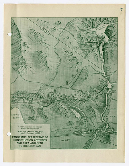
This map shows how the construction of such an engineering feat happens while in progress, having intake, pumps and reservoirs constructed first, then pipeline completed afterward, shown as dotted lines on this 1932 map.

This blog post entry was written by CLIR CCEPS Fellow, Lilyan Rock:

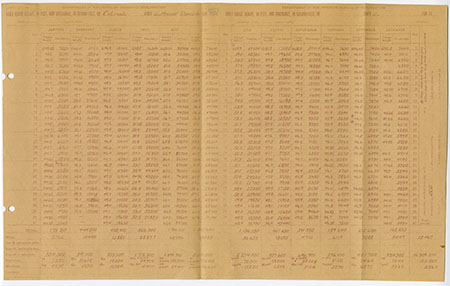
River courses, after carving through the Earth like how the Colorado has done to the Grand Canyon, don’t change coordinates within the span of a century. They can, however, change flow and rate, either naturally or synthetically through the construction of dams and irrigation maneuvering. Environmental historians may find charts such as this one below, worth more than just the values of their numbers.

When measuring the effects of water management on an environment it is important to consider the previously recorded flow of a river, versus the current recorded outputs from today. Not only do environmental historians have to work with scientifically recorded data, to glean said data they must keep up with the changing technologies over the years as well.

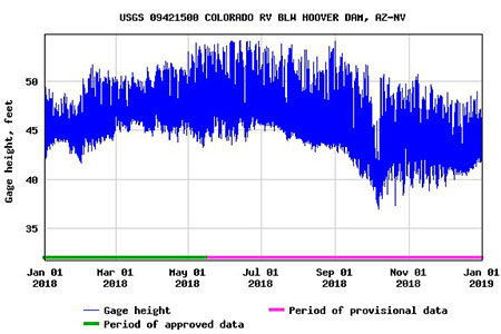
This image above is part of the Boulder Canyon Projects series, charting the average flow between January to December of 1932 at the location of modern day’s Hoover Dam. The chart below is from Hoover Dam’s flow between January to December of 2018.

Normal
0

false
false
false

EN-US
X-NONE
X-NONE

This blog post entry was written by CLIR CCEPS Fellow, Vinh
Tran:

There are lots of
data that can be found in the pile of crumbling papers from the Willis S. Jones
boxes: hydraulic head, rainfall, water flow, soil composition, etc. The thing,
no one really turned them to graphs, probably because of the somewhat monstrous
handwriting (seriously, is that an F, an S, or a P?), lack of measurement units
(also, head of water [ft] or atm, pick one!), and the general unavailability of
our lord and savior, Excel! But now that we can gather and view them in one
place, producing charts and graphs can be easily done and may help us better
understand the geographical and geological characteristics of the region (if
you’re into that kind of stuff). Who knows, someone might actually use them for
their research (not me though). One last thing, who the hell thinks it’s a good
idea to use log_√2 for the x-axis?